Learning Representations by Back-propagating Errors
This is the classic paper that rediscovered back-propagation. Conceptually, back propagation is quite simple and just is a repeated application of chain rule. However, results of applying backprop for multi layer neural networks have been spectacular. This paper reads like a very brief tutorial of deep learning.
Yellow highlights/annotations are my own. You can disable them.Abstract
We describe a new learning procedure, back-propagation, for networks of neurone-like units. The procedure repeatedly adjusts the weights of the connections in the network so as to minimize a measure of the difference between the actual output vector of the net and the desired output vector. As a result of the weight adjustments, internal ‘hidden’ units which are not part of the input or output come to represent important features of the task domain, and the regularities in the task are captured by the interactions of these units. The ability to create useful new features distinguishes back-propagation from earlier, simpler methods such as the perceptron-convergence procedure[1].
Paper
There have been many attempts to design self-organizing neural networks. The aim is to find a powerful synaptic modification rule that will allow an arbitrarily connected neural network to develop an internal structure that is appropriate for a particular task domain. The task is specified by giving the desired state vector of the output units for each state vector of the input units. If the input units are directly connected to the output units it is relatively easy to find learning rules that iteratively adjust the relative strengths of the connections so as to progressively reduce the difference between the actual and desired output vectors[2]. Learning becomes more interesting but more difficult when we introduce hidden units whose actual or desired states are not specified by the task. (In perceptrons, there are ‘feature analysers’ between the input and output that are not true hidden units because their input connections are fixed by hand, so their states are completely determined by the input vector: they do not learn representations.) The learning procedure must decide under what circumstances the hidden units should be active in order to help achieve the desired input-output behaviour. This amounts to deciding what these units should represent. We demonstrate that a general purpose and relatively simple procedure is powerful enough to construct appropriate internal representations.
The simplest form of the learning procedure is for layered networks which have a layer of input units at the bottom; any number of intermediate layers; and a layer of output units at the top. Connections within a layer or from higher to lower layers are forbidden, but connections can skip intermediate layers. An input vector is presented to the network by setting the states of the input units. Then the states of the units in each layer are determined by applying equations (1) and (2) to the connections coming from lower layers. All units within a layer have their states set in parallel, but different layers have their states set sequentially, starting at the bottom and working upwards until the states of the output units are determined.
The total input, $x_j$, to unit $j$ is a linear function of the outputs, $y_i$, of the units that are connected to $j$ and of the weights, $w_{ji}$, on these connections
\[x_j = \sum_i y_i w_{ji} \tag{1}\]Units can be given biases by introducing an extra input to each unit which always has a value of $1$. The weight on this extra input is called the bias and is equivalent to a threshold of the opposite sign. It can be treated just like the other weights.
A unit has a real-valued output, $y_j$, which is a non-linear function of its total input
\[y_j = \frac{1}{1 + e^{-x_j}} \tag{2}\]It is not necessary to use exactly the functions given in equations (1) and (2). Any input-output function which has a bounded derivative will do. However, the use of a linear function for combining the inputs to a unit before applying the nonlinearity greatly simplifies the learning procedure.
The aim is to find a set of weights that ensure that for each input vector the output vector produced by the network is the same as (or sufficiently close to) the desired output vector. If there is a fixed, finite set of input-output cases, the total error in the performance of the network with a particular set of weights can be computed by comparing the actual and desired output vectors for every case. The total error, $E$, is defined as
\[E = \frac{1}{2} \sum_c \sum_j (y_{j,c} - d_{j, c}) ^ 2 \tag{3}\]where $c$ is an index over cases (input-output pairs), $j$ is an index over output units, $y$ is the actual state of an output unit and $d$ is its desired state. To minimize $E$ by gradient descent it is necessary to compute the partial derivative of $E$ with respect to each weight in the network. This is simply the sum of the partial derivatives for each of the input-output cases. For a given case, the partial derivatives of the error with respect to each weight are computed in two passes. We have already described the forward pass in which the units in each layer have their states determined by the input they receive from units in lower layers using equations (1) and (2). The backward pass which propagates derivatives from the top layer back to the bottom one is more complicated.
The backward pass starts by computing $\partial E/\partial y$ for each of the output units. Differentiating equation (3) for a particular case, $c$, and suppressing the index $c$ gives
\[\partial E / \partial y_j = y_j - d_j \tag{4}\]We can then apply the chain rule to compute $\partial E/\partial x_j$
\[\partial E / \partial x_j = \partial E / \partial y_j \cdot dy_j/dx_j\]Differentiating equation (2) to get the value of $dy_j/dx_j$, and substituting gives
\[\partial E / \partial x_j = \partial E / \partial y_j \cdot y_j (1 - y_j) \tag{5}\]This means that we know how a change in the total input $x$ to an output unit will affect the error. But this total input is just a linear function of the states of the lower level units and it is also a linear function of the weights on the connections, so it is easy to compute how the error will be affected by changing these states and weights. For a weight $w_{ji}$, from $i$ to $j$ the derivative is
\[\partial E / \partial w_{ji} = \partial E / \partial x_j \cdot \partial x_j / \partial w_{ji} = \partial E / \partial x_j \cdot y_i \tag{6}\]and for the output of the $i$th unit the contribution to $\partial E/\partial y_i$ resulting from the effect of $i$ on $j$ is simply
\[\partial E / \partial x_{j} \cdot \partial x_j / \partial y_i = \partial E / \partial x_{j} \cdot w_{ji}\]so taking into account all the connections emanating from unit $i$ we have
\[\partial E / \partial y_{i} = \sum_j \partial E / \partial x_{j} \cdot w_{ji} \tag{7}\]We have now seen how to compute $\partial E / \partial y$ for any unit in the penultimate layer when given $\partial E / \partial y$ for all units in the last layer. We can therefore repeat this procedure to compute this term for successively earlier layers, computing $\partial E / \partial w$ for the weights as we go.
One way of using $\partial E / \partial w$ is to change the weights after every input-output case. This has the advantage that no separate memory is required for the derivatives. An alternative scheme, which we used in the research reported here, is to accumulate $\partial E / \partial w$ over all the input-output cases before changing the weights. The simplest version of gradient descent is to change each weight by an amount proportional to the accumulated $\partial E / \partial w$
\[\nabla w = - \varepsilon \partial E / \partial w \tag{8}\]This method does not converge as rapidly as methods which make use of the second derivatives, but it is much simpler and can easily be implemented by local computations in parallel hardware. It can be significantly improved, without sacrificing the simplicity and locality, by using an acceleration method in which the current gradient is used to modify the velocity of the point in weight space instead of its position
\[\nabla w (t) = - \varepsilon \partial E / \partial w (t) + \alpha \nabla w (t-1) \tag{9}\]where $t$ is incremented by 1 for each sweep through the whole set of input-output cases, and $\alpha$ is an exponential decay factor between 0 and 1 that determines the relative contribution of the current gradient and earlier gradients to the weight change.
To break symmetry we start with small random weights. Variants on the learning procedure have been discovered independently by David Parker (personal communication) and by Yann Le Cun[3].
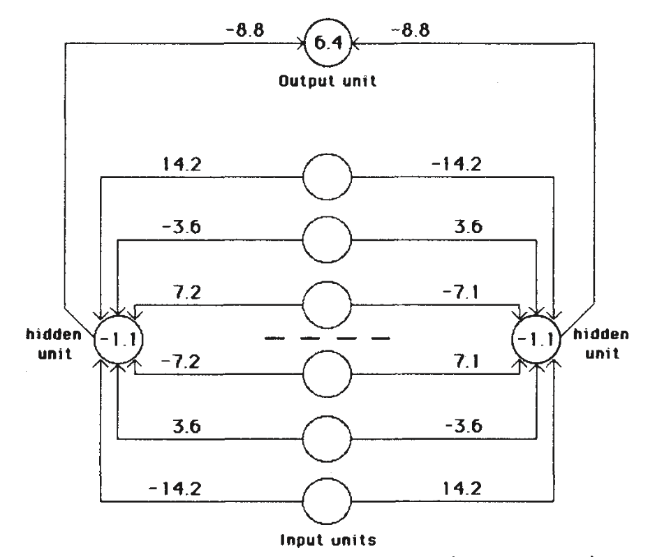
One simple task that cannot be done by just connecting the input units to the output units is the detection of symmetry. To detect whether the binary activity levels of a one-dimensional array of input units are symmetrical about the centre point, it is essential to use an intermediate layer because the activity in an individual input unit, considered alone, provides no evidence about the symmetry or non-symmetry of the whole input vector, so simply adding up the evidence from the individual input units is insufficient. (A more formal proof that intermediate units are required is given in ref.2.) The learning procedure discovered an elegant solution using just two intermediate units, as shown in Fig. 1.
Fig. 1 A network that has learned to detect mirror symmetry in
the input vector. The numbers on the arcs are weights and the numbers inside the nodes are biases. The learning required 1,425 sweeps through the set of 64 possible input vectors, with the weights being adjusted on the basis of the accumulated gradient after each sweep. The values of the parameters in equation (9) were $\varepsilon = 0.1$ and $\alpha = 0.9$. The initial weights were random and were uniformly distributed between -0.3 and 0.3. The key property of this solution is that for a given hidden unit, weights that are symmetric about the middle of the input vector are equal in magnitude and opposite in sign. So if a symmetrical pattern is presented, both hidden units will receive a net input of 0 from the input units, and, because the hidden units have a negative bias, both will be off. In this case the output unit, having a positive bias, will be on. Note that the weights on each side of the midpoint are in the ratio 1:2:4. This ensures that each of the eight patterns that can occur above the midpoint sends a unique activation sum to each hidden unit, so the only pattern below the midpoint that can exactly balance this sum is the symmetrical one. For all non-symmetrical patterns, both hidden units will receive non-zero activations from the input units. The two hidden units have identical patterns of weights but with opposite signs, so for every non-symmetric pattern one hidden unit will come on and suppress the output unit.
Another interesting task is to store the information in the two family trees (Fig. 2). Figure 3 shows the network we used, and Fig. 4 shows the ‘receptive fields’ of some of the hidden units after the network was trained on 100 of the 104 possible triples.
Fig. 2 Two isomorphic family trees. The information can be expressed as 4 set of triples of the form ⟨person 1⟩⟨relationship⟩⟨person 2⟩, where the possible relationships are {father, mother, husband, wife, son, daughter, uncle, aunt, brother, sister, nephew, niece}. A layered net can be said to ‘know’ these triples if it can produce the third term of each triple when given the first two. The first two terms are encoded by activating two of the input units, and the network must then complete the proposition by activating the output unit that represents the third term.
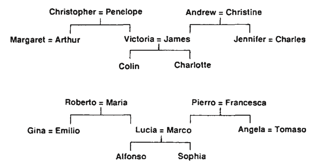
Fig. 3 Activity levels in a five-laver network after it has learned, The bottom layer has 24 input units on the left for representing ⟨person 1⟩ and 12 input units an the right for representing the relationship. The white squares inside these two groups show the activity levels of the units. There is one active unit in the first group representing Colin and one in the second group representing the relationship ‘has-aunt’. Each of the two input groups is totally connected to its own group of 6 units in the second layer. These groups learn to encode people and relationships as distributed patterns of activity. The second layer is totally connected to the central layer of 12 units, and these are connected to the penultimate layer of 6 units. The activity in the penultimate layer must activate the correct output units, each of which stands for a particular (person 2). In this case, there are two correct answers (marked by black dots) because Colin has two aunts. Both the input units and the output units are laid out spatially with the English people in one row and the isomorphic Italians immediately below.
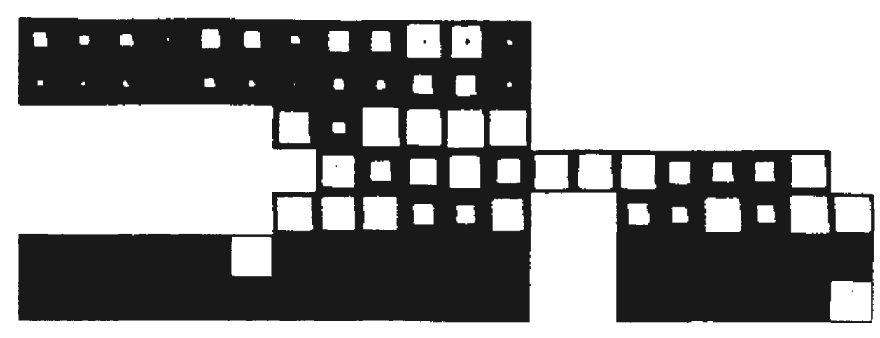
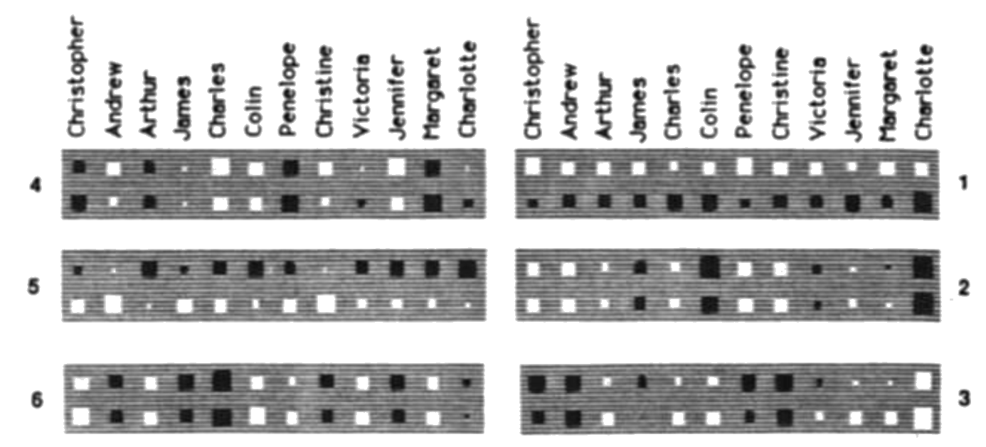
Fig. 4 The weights from the 24 input units that represent people to the 6 units in the second layer that learn distributed representations of people. White rectangles, excitatory weights; black rectangles, inhibitory weights; area of the rectangle encodes the magnitude of the weight. The weights from the 12 English people are in the top row of each unit. Unit 1 is primarily concerned with the distinction between English and Italian and most of the other units ignore this distinction. This means that the representation of an English person is very similar to the representation of their Italian equivalent. The network is making use of the isomorphism between the two family trees to allow it to share structure and it will therefore tend to generalize sensibly from one tree to the other. Unit 2 encodes which generation a person belongs to, and unit 6 encodes which branch of the family they come from. The features captured by the hidden units are not at all explicit in the input and output encodings, since these use a separate unit for each person. Because the hidden features capture the underlying structure of the task domain, the network generalizes correctly to the four triples on which it was not trained. We trained the network for 1500 sweeps, using $\varepsilon = 0.005$ and $\alpha =0.5$ for the first 20 sweeps and $\varepsilon = 0.001$ and $\alpha =0.9$ for the remaining sweeps. To make it easier to interpret the weights we introduced ‘weight-decay’ by decrementing every weight by 0.2% after each weight change. After prolonged learning, the decay was balanced by $\partial E / \partial w$, so the final magnitude of each weight indicates its usefulness in reducing the error. To prevent the network needing large weights to drive the outputs to 1 or 0, the error was considered to be zero if output units that should be on had activities above 0.8 and output units that should be off had activities below 0.2.
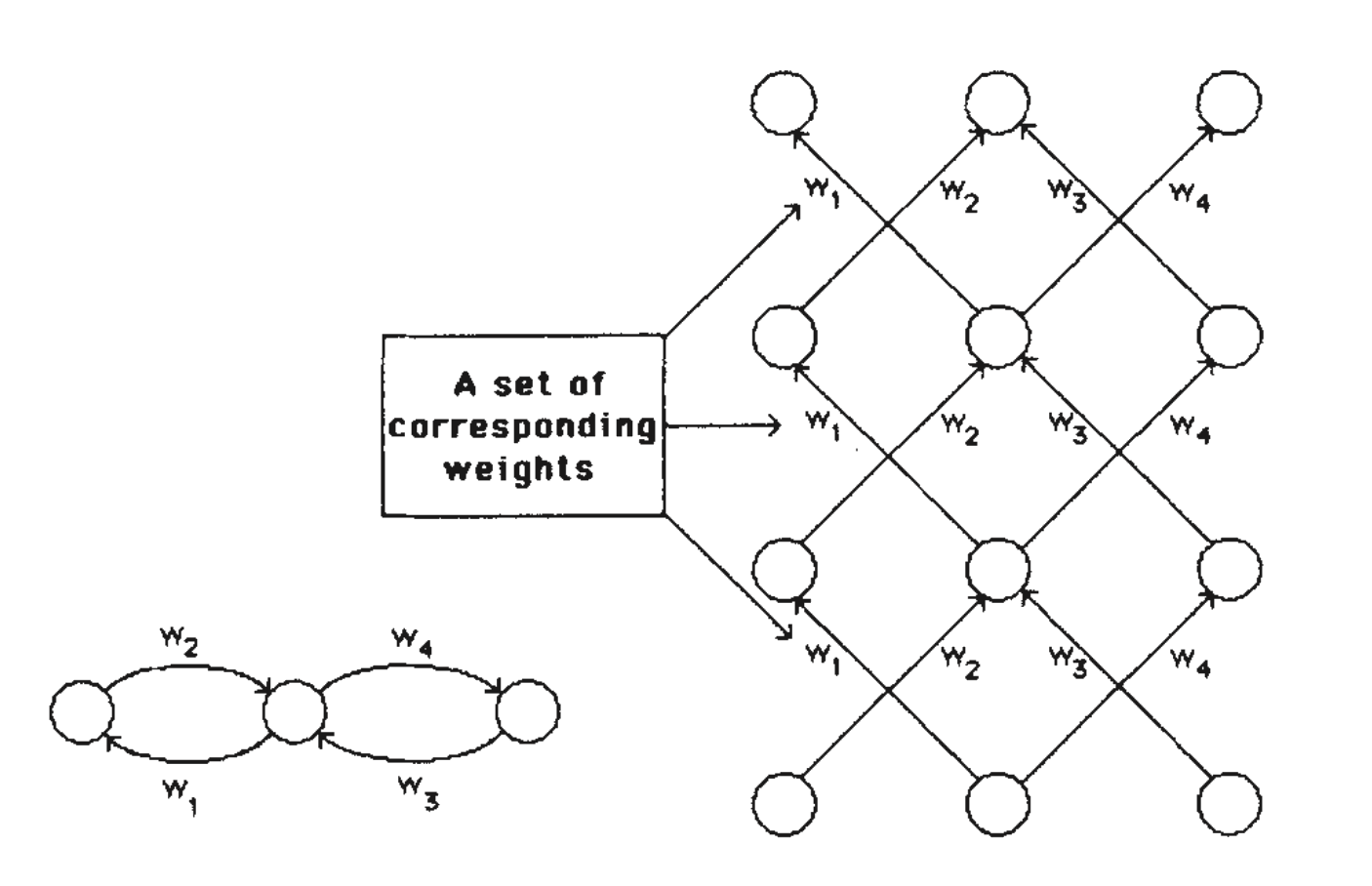
So far, we have only dealt with layered, feed-forward networks. The equivalence between layered networks and recurrent networks that are run iteratively is shown in Fig. 5.
The most obvious drawback of the learning procedure is that the error-surface may contain local minima so that gradient descent is not guaranteed to find a global minimum. However, experience with many tasks shows that the network very rarely gets stuck in poor local minima that are significantly worse than the global minimum. We have only encountered this undesirable behaviour in networks that have just enough connections to perform the task. Adding a few more connections creates extra dimensions in weight-space and these dimensions provide paths around the barriers that create poor local minima in the lower dimensional subspaces.
The learning procedure, in its current form, is not a plausible model of learning in brains. However, applying the procedure to various tasks shows that interesting internal representations can be constructed by gradient descent in weight-space, and this suggests that it is worth looking for more biologically plausible ways of doing gradient descent in neural networks.
Fig. 5 A synchronous iterative net that is run for three iterations and the equivalent layered net. Each time-step in the recurrent net corresponds to a layer in the layered net. The learning procedure for layered nets can be mapped into a learning procedure for iterative nets. Two complications arise in performing this mapping: first, in a layered net the output levels of the units in the intermediate layers during the forward pass are required for performing the backward pass (see equations (5) and (6)). So in an iterative net it is necessary to store the history of output states of each unit. Second, for a layered net to be equivalent to an iterative net, corresponding weights between different layers must have the same value. To preserve this property, we average $\partial E / \partial w$ for all the weights in each set of corresponding weights and then change each weight in the set by an amount proportional to this average gradient. With these two provisos, the learning procedure can be applied directly to iterative nets. These nets can then either learn to perform
iterative searches or learn sequential structures[4].
We thank the System Development Foundation and the Office of Naval Research for financial support.
References:
- Rosenblatt, F. Principles Of Neurodynamics (Spartan, Washington, DC, 1961}.
- Minsky, M. L. & Papert, S. Perceptrons (MIT, Cambridge, 1969).
- Le Cun, Y, Proc. Cognitiva 85, 599-804 (1985).
- Rumelhart, D. E., Hinton, G. E. & Williams, R. J. in Parallel Distributed Processing: Expliorations in the Mi fare of Cognition, Vol. i: Foundations (eds Rumelhart, D. E. & McClelland, J L.} 318-382 (MIT, Cambridge, 1986).