Deep Learning Crash Course Part 2

Sasank Chilamkurthy | 16 May 2017 | 17 minutes to read.

Continued from Part 1. We have so far seen MLPs and why they are hard to train. Now, we will develop networks which overcome these difficulties.

Convolutional Neural Networks

Let’s go back to the problem of handwritten digit recognition. MLP looks like this:

Figure: MLP for MNIST. Source.

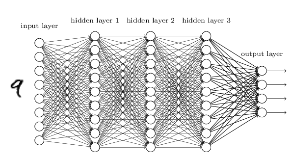
In particular, we have connected all the pixels in 28x28 images i.e, 784 pixels to each neuron in hidden layer 1.

Upon reflection, it’s strange to use networks with fully-connected layers to classify images. The reason is that such a network architecture does not take into account the spatial structure of the images. For instance, it treats input pixels which are far apart and close together on exactly the same footing. Such concepts of spatial structure must instead be inferred from the training data.

But what if, instead of starting with a network architecture which is tabula rasa, we used an architecture which tries to take advantage of the spatial structure? In this section I describe convolutional neural networks. These networks use a special architecture which is particularly well-adapted to classify images. Using this architecture makes convolutional networks fast to train. This, in turn, helps us train deep, many-layer networks, which are very good at classifying images. Today, deep convolutional networks or some close variant are used in most neural networks for image recognition.

Convolutional neural networks use three basic ideas:

Local receptive fields
Shared weights
Pooling.

Local receptive fileds

As per usual, we’ll connect the input pixels to a layer of hidden neurons. But we won’t connect every input pixel to every hidden neuron. Instead, we only make connections in small, localized regions of the input image.

Figure: Local receptive fields of convolution. Source.

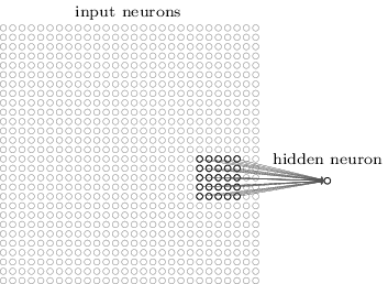
That region in the input image is called the local receptive field for the hidden neuron. It’s a little window on the input pixels. Each connection learns a weight. And the hidden neuron learns an overall bias as well. You can think of that particular hidden neuron as learning to analyze its particular local receptive field.

We then slide the local receptive field across the entire input image. For each local receptive field, there is a different hidden neuron in the first hidden layer. To illustrate this concretely, let’s start with a local receptive field in the top-left corner:

Figure: Convolution. Source.

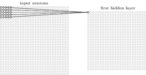
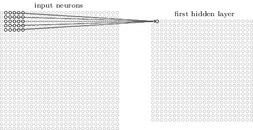
Then we slide the local receptive field over by one pixel Sometimes a different stride length (e.g, 2) is used. to the right (i.e., by one neuron), to connect to a second hidden neuron Note that if we have a 28×28 input image, and 5×5 local receptive fields, then there will be 24×24 neurons in the hidden layer. :

Figure: Slide the convolution. Source.

Shared weights and biases

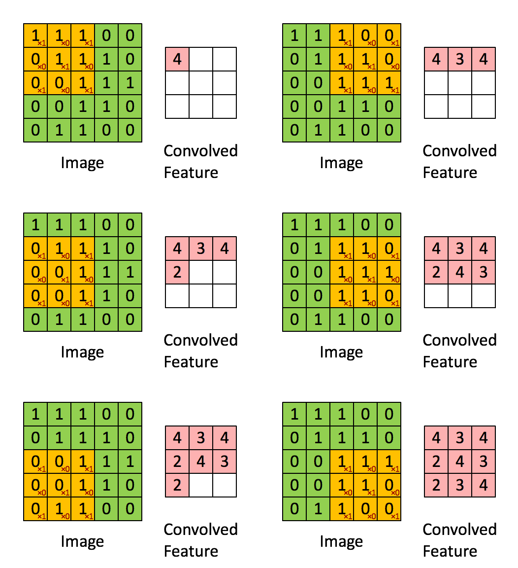
I’ve said that each hidden neuron has a bias and 5×5 weights connected to its local receptive field. What I did not yet mention is that we’re going to use the same weights and bias for each of the 24×24 hidden neurons.

Following animation makes the schematic of convolution clear:

Figure: Convolution Schematic. Note that biases are not shown here. Source.

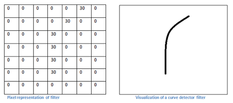
Sharing weights and biases means that all the neurons in the first hidden layer detect exactly the same feature just at different locations in the input image. To see why this makes sense, consider the following convolution filter:

Figure: A convolutional filter. Source.

Let’s take an example image and apply convolution on a receptive filed:

Figure: Convolution on an example image. Source.

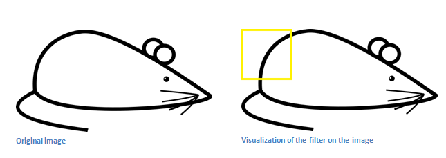
Figure: Apply convolution. Source.

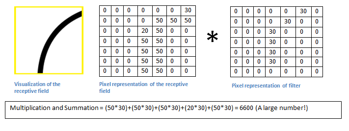
Basically, in the input image, if there is a shape that generally resembles the curve that this filter is representing, then all of the multiplications summed together will result in a large value! Now let’s see what happens when we move our filter.

Figure: Apply convolution at a different receptive field. Source.

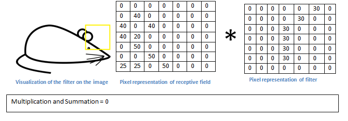
Therefore, this convolution picks up a right bending curve wherever it is on . To put it in slightly more abstract terms, convolutional networks are well adapted to the translation invariance of images: move a picture of a cat (say) a little ways, and it’s still an image of a cat

The network structure I’ve described so far can detect just a single kind of localized feature. To do image recognition we’ll need more than one feature map. And so a complete convolutional layer consists of several different feature maps

Figure: Multiple feature maps. Source.

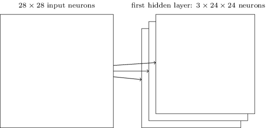
A big advantage of sharing weights and biases is that it greatly reduces the number of parameters involved in a convolutional network. For each feature map we need 25=5×5 shared weights, plus a single shared bias. So each feature map requires 26 parameters. If we have 20 feature maps that’s a total of 20×26=520 parameters defining the convolutional layer. By comparison, suppose we had a fully connected first layer, with 784=28×28 input neurons, and a relatively modest 30 hidden neurons. That’s a total of 784×30 weights, plus an extra 30 biases, for a total of 23,550 parameters.

Pooling layers

In addition to the convolutional layers just described, convolutional neural networks also contain pooling layers. Pooling layers are usually used immediately after convolutional layers. What the pooling layers do is simplify the information in the output from the convolutional layer.

In detail, a pooling layer takes each feature map output from the convolutional layer and prepares a condensed feature map. For instance, each unit in the pooling layer may summarize a region of (say) 2x2 neurons in the previous layer. As a concrete example, one common procedure for pooling is known as max-pooling. In max-pooling, a pooling unit simply outputs the maximum activation in the 2x2 input region, as illustrated in the following diagram:

Figure: Pooling Layer. Source.

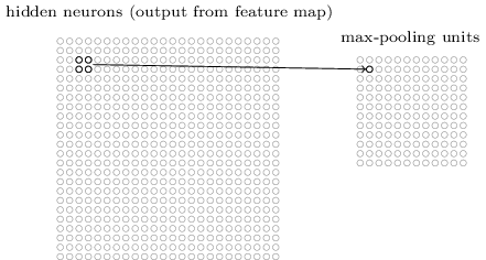
Note that since we have 24×24 neurons output from the convolutional layer, after pooling we have 12×12 neurons.

As mentioned above, the convolutional layer usually involves more than a single feature map. We apply max-pooling to each feature map separately. So if there were three feature maps, the combined convolutional and max-pooling layers would look like:

Figure: Convolution and pooling layer. Source.

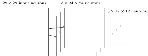
We can think of max-pooling as a way for the network to ask whether a given feature is found anywhere in a region of the image. It then throws away the exact positional information. The intuition is that once a feature has been found, its exact location isn’t as important as its rough location relative to other features. A big benefit is that there are many fewer pooled features, and so this helps reduce the number of parameters needed in later layers.

Case Study: LeNet

Let’s put everything we’ve learnt together and analyze one of the very early successesLeNet is published in 1998! CNNs are not exactly new. of convolutional networks: LeNet. This is the architecture of LeNet:

Figure: LeNet architecture Source.

Let’s go over each of the component layers of LeNet: I actually describe slightly modified version of LeNet.

Input: Gray scale image of size 32 x 32.
C1: Convolutional layer of 6 feature maps, kernel size (5, 5) and stride 1. Output size therefore is 6 X 28 x 28. Number of trainable parameters is $(5*5 + 1) * 6 = 156$.
S2: Pooling/subsampling layer with kernel size (2, 2) and stride 2. Output size is 6 x 14 x 14. Number of trainable parameters = 0.
C3: Convolutional layer of 16 feature maps. Each feature map is connected to all the 6 feature maps from the previous layer. Kernel size and stride are same as before. Output size is 16 x 10 x 10. Number of trainable parameters is $(6 * 5 * 5 + 1) * 16 = 2416$.
S4: Pooling layer with same hyperparameters as above. Output size = 16 x 5 x 5.
C5: Convolutional layer of 120 feature maps and kernel size (5, 5). This amounts to full connection with outputs of previous layer. Number of parameters are $(16 * 5 * 5 + 1)*120 = 48120$.
F6: Fully connected layer of 84 units. i.e, All units in this layer are connected to previous layer’s outputsThis is same as layers in MLP we’ve seen before.. Number of parameters is $(120 + 1)*84 = 10164$
Output: Fully connected layer of 10 units with softmax activationIgnore ‘Gaussian connections’. It is for a older loss function no longer in use..

Dataset used was MNIST. It has 60,000 training images and 10,000 testing examples.

Tricks of the Trade

Dropout

With so many parameters in neural networks, overfitting is a real problem. For example, LeNet has about the same number of parameters as there are training examples. There are a few techniques like $L_1$/$L_2$ regularization you might be familiar with. These modify cost function by adding $L_1$/$L_2$ norm of parameters respectively.

Dropout is radically different for regularization. We modify the network itself instead of the cost function. Suppose we’re trying to train a network:

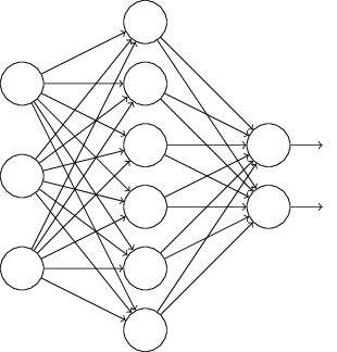
With dropout, We start by randomly (and temporarily) deleting half the hidden neurons in the network, while leaving the input and output neurons untouched. After doing this, we’ll end up with a network along the following lines.

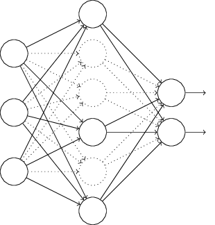
We forward-propagate the input $x$ through the modified network, and then backpropagate the result, also through the modified network. After doing this over a mini-batch of examples, we update the appropriate weights and biases. We then repeat the process, first restoring the dropout neurons, then choosing a new random subset of hidden neurons to delete, estimating the gradient for a different mini-batch, and updating the weights and biases in the network.

The weights and biases will have been learnt under conditions in which half the hidden neurons were dropped out. When we actually run the full network that means that twice as many hidden neurons will be active. To compensate for that, we halve the weights outgoing from the hidden neurons.

Why would dropout help? Explanation from AlexNet paper AlexNet is the paper which lead to renaissance of CNNs.:

This technique reduces complex co-adaptations of neurons, since a neuron cannot rely on the presence of particular other neurons. It is, therefore, forced to learn more robust features that are useful in conjunction with many different random subsets of the other neurons.

In other words, we can think of dropout as a way of making sure that the model is robust to the loss of any individual piece of evidence. Of course, the true measure of dropout is that it has been very successful in improving the performance of neural networks.

Data Augmentation

You probably already know that more data leads to better accuracy. It’s not surprising that this is the case, since less training data means our network will be exposed to fewer variations in the way human beings write digits.

Obtaining more training data can be expensive, and so is not always possible in practice. However, there’s another idea which can work nearly as well, and that’s to artificially expand the training data. Suppose, for example, that we take an MNIST training image of a five,

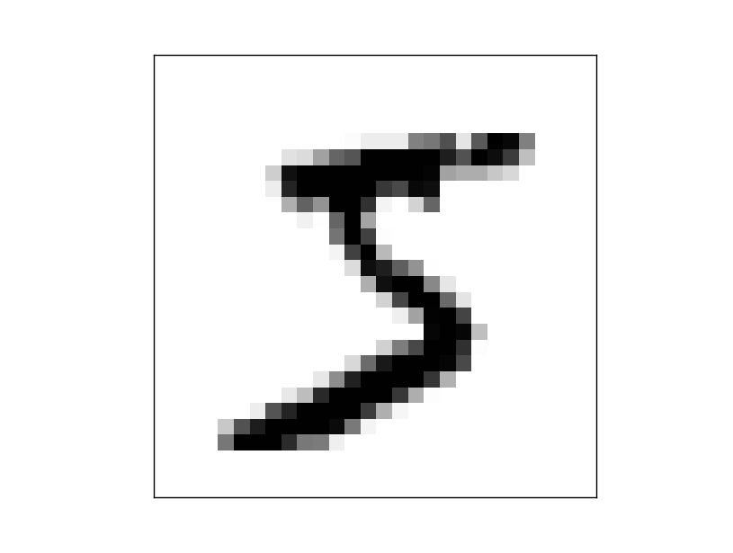
and rotate it by a small amount, let’s say 15 degrees:

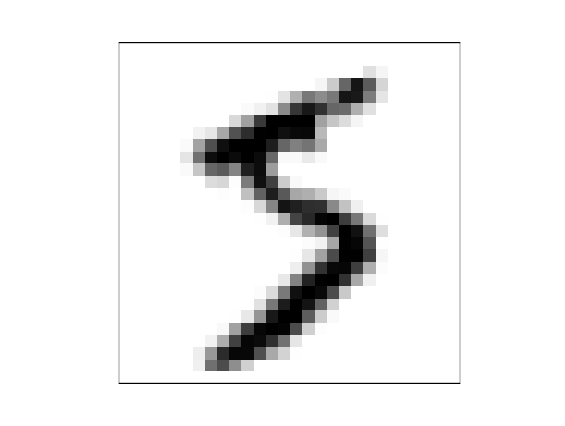
It’s still recognizably the same digit. And yet at the pixel level it’s quite different to any image currently in the MNIST training data. We can expand our training data by making many small rotations of all the MNIST training images, and then using the expanded training data to improve our network’s performance.

We call such expansion as data augmentation. Rotation is not the only way to augment the data. A few examples are crop, zoom etc. The general principle is to expand the training data by applying operations that reflect real-world variation.

Weight initialization and Batch Normalization

Training neural networks is a highly non convex problem. Therefore, initialization of parameters to be optimized is important. To understand better, recall the unstable gradient problem. This is the equation of gradients for parameters in $j$th layer:

\[\frac{\partial C}{\partial \theta_l} = \frac{\partial y_L}{\partial u_L} * \frac{\partial y_{L-1}}{\partial u_{L-1}} * \cdots * \frac{\partial y_{l-1}}{\partial u_{l-1}} * \frac{\partial y_l}{\partial \theta_l}\]

If each layer is not properly initialized, scales inputs by $k$, i.e $\frac{\partial y_m}{\partial u_m} \approx k$. Therefore gradients of parameters in $l$ th layer is

\[\frac{\partial C}{\partial \theta_l} = k^{L - l}\]

Thus, $k > 1$ leads to extremely large gradients and $k<1$ to very small gradients in initial layers. Therefore, we want

\[k \approx 1\]

This can be made sure with good weight initialization. Historically, bad weight inits are what prevented deep neural networks to be trained.

A recently developed technique called Batch Normalization alleviates a lot of headaches with initializations by explicitly forcing this throughout a network. The core observation is that this is possible because normalization is a simple differentiable operation.

It has become a very common practice to use Batch Normalization in neural networks. In practice, networks that use Batch Normalization are significantly more robust to bad initialization.

Practical Advice

ImageNet Dataset and ILSVRC

ImageNet is a huge dataset for visual recognition research. It currently has about 14 million images tagged manually.

ImageNet project runs an annual software contest, the ImageNet Large Scale Visual Recognition Challenge (ILSVRC), where software programs compete to correctly classify and detect objects and scenes. ILSVRC recognition challenge is conducted on a subset of ImageNet: 1.2 million images with 1000 classes.

Here are example images and the recognition results:

Figure: Images from imagenet. Source.

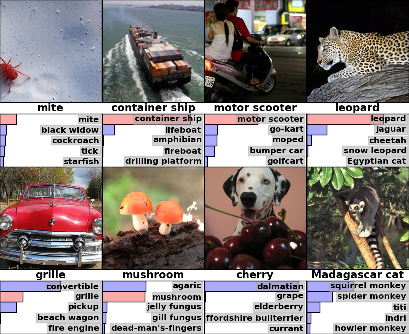
Alexnet was the first CNN to participate in ILSVRC and won the 2012 challenge by a significant margin. This lead to a renaissance of CNNs for visual recognition. This is the architecture:

Figure: Alexnet architecture. Source.

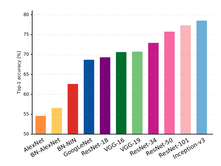
It isn’t too different from LeNet we discussed before. Over the years, newer CNN architectures won this challenge. Notable ones are

VGGNet
GoogLeNet
Inception
ResNet

You will keep on hearing these architectures if work more on CNNs. Here are the accuracies from these networks:

Figure: Top 1 accuracies on ILSVRC. Source.

Transfer Learning

To train a CNNs like above from scratch (i.e random initialization), you will need a huge dataset of the ImageNet scale. In practice, very few people do this.

Instead, you will pretrain your network on large dataset like imagenet and use the learned weights as initializations. Usually, you will just download the trained model of one of the above architectures from internet and use them as your weight initializations. This is called transfer learning.

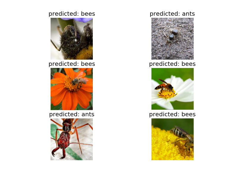
This is a very powerful trick. For example, here I used pretrained weights of ResNet-18 and trained a classifier to classify ants and bees.

Figure: Ants/Bees classifier. Source.

My dataset:

Training: 120 ants + 120 bees images
Testing: 75 ants + 75 bees images

With this small dataset, I got around 95 % accuracy!

Why does transfer learning work? 1.2 million images in imagenet cover wide diversity of real world images. Filters learned on imagenet will therefore be sufficiently general to apply on any similar problem. i.e, you will not overfit on your small dataset.

Moral of the story: you don’t need a large dataset if you are working on real life images!

GPUs

GPUs dramatically speed up neural networks. This is because most of the neural network computation is just matrix multiplication and thus is readily vectorizable. GPUs excel at such computations.

For example, look at the times taken by my transfer learning code to train:

~ 20 min on CPU
~ 1 min on GPU

And this was with meager dataset of 400 images. Imagine working with a dataset of the scale of ImageNet. GPUs are essential if you are serious about deep learning.

Other FAQ

What framework to use?

Lot of frameworks are available: Keras, Tensorflow, PyTorch. I suggest using Keras if you are new to deep learning.

How do I know what architecture to use?

Don’t be a hero! - Andrej Karpathy

Take whatever works best on ILSVRC (latest ResNet)

Download a pretrained model

Potentially add/delete some parts of it

Finetune it on your application.

How do I know what hyperparameters to use?

Don’t be a hero! - Andrej Karpathy

Use whatever is reported to work best on ILSVRC.

Play with the regularization strength (dropout rates)

But my model is not converging!

Take a very small subset (like, 50 samples) of your dataset and train your network on this.

Your network should completely overfit on this data. If not play with learning rates. If you couldn’t get your network to overfit, something is either wrong with your code/initializations or you need to pick a powerful model.